
The building model is calculated in two phases:
- Global 3D calculation of the global model, where the slabs are modeled as a rigid plane (diaphragm) or as a bending plate
- Local 2D calculation of the individual floors
After the calculation, the results of the columns and walls from the 3D calculation and the results of the slabs from the 2D calculation are combined in a single model. This means that there is no need to switch between the 3D model and the individual 2D models of the slabs. The user only works with one model, saves valuable time, and avoids possible errors in the manual data exchange between the 3D model and the individual 2D ceiling models.
The vertical surfaces in the model can be divided into shear walls and opening lintels. The program automatically generates internal result members from these wall objects, so they can be designed as members according to any standard in the Concrete Design add-on.
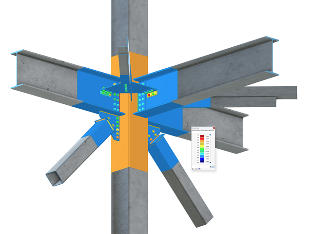
Complex Connection of Horizontal Beams to Column and Connection of Reinforcing Diagonals
The connection model was modeled using about 50 components. The model was created according to the real example of use in structure.
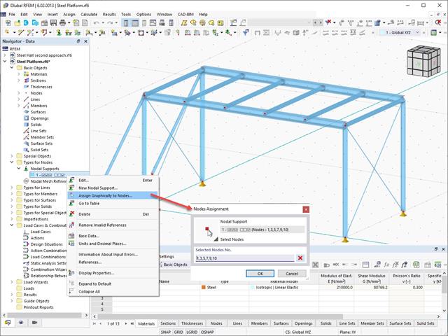
The object types listed below can be graphically assigned to the elements of the structure modeled in the program.
- Nodal supports
- Member shear panels
- Local reductions of member cross-sections
- Member transverse stiffeners
- Member longitudinal welds
- Effective lengths
- Boundary conditions
- Line supports
- Loads
- Member support
- Punching reinforcements
- Mesh refinements
- Surface reinforcements
- Surface results adjustments
- Surface support
- Service classes
- Imperfections

Did you know? In contrast to other material models, the stress-strain diagram for this material model is not antimetric to the origin. You can use this material model to simulate the behavior of steel fiber-reinforced concrete, for example. Find detailed information about modeling steel fiber-reinforced concrete in the technical article about Determining the material properties of steel-fiber-reinforced concrete.
In this material model, the isotropic stiffness is reduced with a scalar damage parameter. This damage parameter is determined from the stress curve defined in the Diagram. The direction of the principal stresses is not taken into account. Rather, the damage occurs in the direction of the equivalent strain, which also covers the third direction perpendicular to the plane. The tension and compression area of the stress tensor is treated separately. In this case, different damage parameters apply.
The "Reference element size" controls how the strain in the crack area is scaled to the length of the element. With the default value zero, no scaling is performed. Thus, the material behavior of the steel fiber concrete is modeled realistically.
Find more information about the theoretical background of the "Isotropic Damage" material model in the technical article describing the Nonlinear Material Model Damage.
- For a new connection model, you have to select a node in the RFEM model
- After selecting a node, the members connected to the node are automatically recognized and assigned
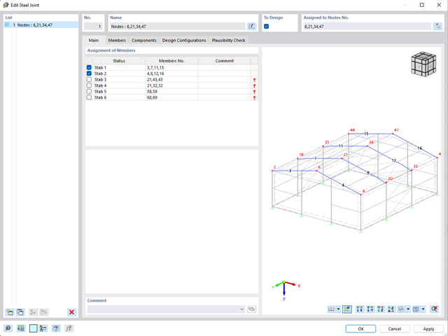
- In the window for assigning members, select the ones that will be assigned to the connection
- The members marked by us are displayed in the preview window on the right
- Connections can be modeled for multiple nodes in a structure.
- For member settings, select the ones to be supported
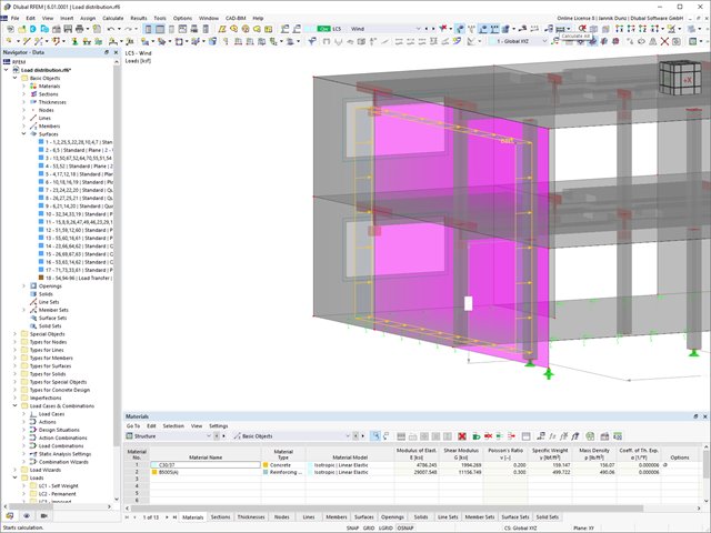
Keep an eye on all surfaces. A surface with the "Load Transfer" stiffness type has no structural effect. You can use it to consider the loads from surfaces that have not been modeled, for example, facade structures, glass surfaces, trapezoidal roof sections, and so on.
Go to Explanatory VideoThe program can also help you here. It determines the bolt forces on the basis of the calculation on the FE model and evaluates them automatically. You can perform the design checks of the bolt resistance for the failure cases tension, shear, hole bearing, and punching shear according to the standard. The program takes care of everything else in this step. It determines all the necessary coefficients and displays them clearly.
- Do you want to perform weld design? The required stresses are also determined on the FE model in that case. Then, the Weld element is modeled as elastic-plastic shell element, where every FE element is checked for its internal forces. (Plasticity criteria is set to reflect failure acc. to AISC J2-4 and J2-5 (weld resistance check) and also J2-2 (base metal capacity check). The design can also be carried out with the partial safety factors according to the selected National Annex.
You can perform the plate design plasticall by comparing the existing plastic strain to the allowable plastic strain. By default this is set to 5% for the AISC 360 but can be specified through user-definition 5% according to EN 1993-1-5, Annex C, or again, user-defined specification.
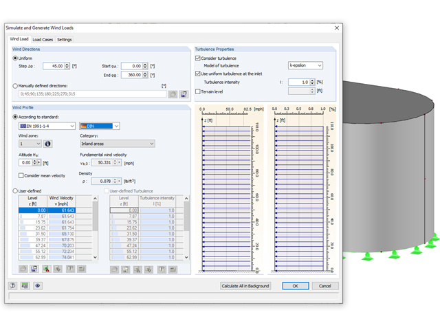
Rely on the Dlubal programs even in windy matters. RFEM and RSTAB provide a special interface for exporting models (that is, structures defined by members and surfaces) to RWIND 2. There, the wind directions to be analyzed for your project are defined by means of related angular positions about the vertical model axis. Furthermore, the elevation-dependent wind profile and turbulence intensity profile are defined on the basis of a wind standard. These specifications result in specific load cases, depending on the angle. For this, the fluid parameters, turbulence model properties, and iteration parameters that are all stored globally are helpful. You can extend these load cases by partial editing in the RWIND 2 environment using terrain or environment models from STL vector graphics.
As an alternative, you can also run RWIND 2 manually and without the interface application in RFEM or RSTAB. In this case, the structures and terrain environment in the program are directly modeled by imported STL and VTP files. You can define the height-dependent wind load and other fluid-mechanical data directly in RWIND 2.
Due to its versatile applicability, RWIND 2 is always at your side to support you in your individual projects.
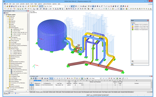
After activating the RF‑PIPING add‑on module, a new toolbar is available in RFEM and the project navigator and tables are extended. The piping system is now modeled in the same way as the members. Pipe bends are defined simultaneously by tangents (straight pipe sections) and radius. Thus, it is easy to subsequently change bend parameters.
It is also possible to extend the piping subsequently by defining special components (expansion joints, valves, and others). The implemented libraries of structural components facilitate the definition.
Continuous pipe sections are defined as sets of piping systems.
For piping loads, member loads are assigned to the respective load cases. The combination of loads is included in piping load combinations and result combinations.
After the calculation, you can display deformations, member internal forces, and support forces graphically or in tables.
Pipe stress analysis according to standards can then be performed in the RF‑PIPING Design add‑on module. You only need to select the relevant sets of piping systems and load situations.
The global calculation assigns the stiffness determined by means of the selected composition and the glass geometry to each surface. Then, the calculation proceeds using the plate theory. It is possible to select whether the shear coupling of layers should be considered.
In the case of the local calculation, you can further specify 2D or 3D calculation. Two-dimensional calculation means that the single-layer or laminated glass is modeled as a surface, whose thickness is calculated on the basis of the selected structure and glass geometry (using the plate theory). Similarly to the global calculation, you can optionally consider shear coupling of layers.
The 3D calculation uses solids in the model to substitute each composition layer. This way, the results are more accurate, but the calculation may take more time.
It is possible to model insulating glass only if local calculation is selected. The gas layer is always modeled as a solid element, so it is necessary to design individual insulating glass parts independently of the surrounding structure. The ideal gas law (thermal equation of state of ideal gases) is considered for the calculation and the third-order analysis.
Initially, it is necessary to define material data, panel dimensions, and boundary conditions (hinged, built-in, unsupported, hinged-elastic). It is possible to transfer the data from RFEM/RSTAB. Then, boundary stresses can be either defined for each load case manually or imported from RFEM/RSTAB.
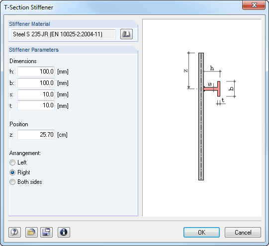
Stiffeners are modeled as spatially effective surface elements that are eccentrically connected to the plate. Therefore, it is not necessary to consider the stiffener eccentricities by effective widths. The bending, shear, strain, and St. Venant stiffness of stiffeners as well as the Bredt stiffness of closed stiffeners is determined automatically in a 3D model.